Introduction
The Risk Analysis and Virtual ENviroment (RAVEN) mission is to provide a framework/container
of capabilities for engineers and scientists to analyze the response of systems, physics and multi-
physics, employing advanced numerical techniques and algorithms. RAVEN was conceived with
two major objectives:
to be as easy and straightforward to use by scientists and engineers as possible.
to allow its expansion in a straightforward manner, providing clear and modular APIs to
developers.
The RAVEN software is meant to be approachable by any type of user (computational scien-
tists, engineers and analysts). Every single aspect of RAVEN was driven by this singular principle
from the build system to the APIs to the software development cycle and input syntax.
The main idea behind the design of the RAVEN software was/is the creation of a multi-purpose
framework characterized by high flexibility with respect to the possible perform-able analysis. The
framework must be capable of constructing the analysis/calculation flow at run-time, interpreting
the user-defined instructions and assembling the different analysis tasks following a user speci-
fied scheme. In order to achieve such flexibility, combined with reasonably fast development, a
programming language naturally suitable for this kind of approach was needed: Python. Hence,
RAVEN is coded in Python and is characterized by an object-oriented design.
System Structure
The core of the analysis perform-able through RAVEN is represented by a set of basic entities
(components/objects) the user can combine, in order to create a customized analysis flow.
Figure 1 shows a schematic representation of the RAVEN software, highlighting the communica-
tion pipes among the different modules and engines.
A list of these components and a summary of their most important characteristics are reported as
follows:
- Distributions: Aimed to explore the input/output space of a system/physics. RAVEN re-
quires the capability to perturb the input space (initial conditions and/or model coefficients
of a system). The input space is generally characterized by probability distribution (density)
functions (PDFs), which might need to be considered when a perturbation is applied. In this
respect, a large library of PDFs is available.
- Samplers: Aimed to define the strategy for perturbing the input space of a system/physics.
A proper approach to sample the input space is fundamental for the optimization of the
computational time. In RAVEN, a “sampler” employs a unique perturbation strategy that is
applied to the input space of a system. The input space is defined through the connection
of uncertain variables (initial conditions and/or model coefficients of a system) and their
relative probability distributions. The link of the input space to the relative distributions,
will allow the Sampler to perform a probability-weighted exploration.
- Optimizers: Aimed to define the strategy for optimizing (constrained or unconstrained) the
controllable input space (parameters) in order to minimize/maximize an objective function
of the system/physics under examination. In RAVEN, an “optimizer” employs an active
learning process (feedback from the underlying model/system/physics) aimed to accelerate
the minimization/maximization of an objective function.
- Models: A model is the representation of a physical system (e.g. Nuclear Power Plant); it is
therefore capable of predicting the evolution of a system given a coordinate set in the input
space. In addition it can represent an action on a data in order to extract key features (e.g.
Data mining).
DataObjects and Databases: Aimed to provide standardized APIs for storing the results of
any RAVEN analysis (Sampling, Optimization, Statistical Analysis, etc.). In addition, these
storage structures represent the common “pipe network” among any entity in RAVEN.
Outstreams: Aimed to export the results of any RAVEN analysis (Sampling, Optimization,
Statistical Analysis, etc.). This entity allows to expose the results of an analysis to the user,
both in text-based (XML, CSV, etc.) or graphical (pictures, graphs, etc.) output files.
Steps: Aimed to provide a standardized way for the user to combine the entities reported
above for the construction of any particular analysis. As shown in Fig. 1, the Step is the
core of the calculation flow of RAVEN and is the only system that is aware of any component
of the simulation.
Job Handler: Aimed to coordinate and regulate the dispatch of jobs in the RAVEN soft-
ware. It is able to monitor/handle parallelism in the driven Models, to interact with High
Performance Computing systems, etc.
Probability Distributions
As already mentioned, the exploration of the input space, through the initial conditions (parameters) affected by uncertainties, needs to be performed using the proper distribution functions. RAVEN provides, through an interface to the BOOST library, the following univariate (truncated and not) distributions: Bernoulli, Binomial, Exponential, Logistic, Lognormal, Normal, Poisson, Triangular, Uniform, Weibull, Gamma, and Beta. The usage of univariate distributions for sampling initial conditions is based on the assumption that the uncertain parameters are not correlated with each other. Quite often uncertain parameters are subject to correlations and thus the univariate approach is not applicable. This happens when the value of multiple initial values are not independent but statistically correlated. RAVEN supports N-dimensional (N-D) PDFs. The user can provide the distribution values on either Cartesian or sparse grid, which determines the interpolation algorithm used in the evaluation of the imported CDF-PDF, respectively:
N-Dimensional Spline, for Cartesian grids
Inverse weight, for sparse grids
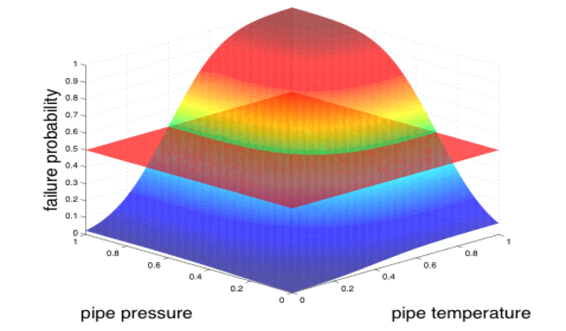
Internally, RAVEN provides the needed N-D differentiation or integration algorithms to compute the PDF from the CDF and vice versa. As already mentioned, the sampling methods use the distributions in order to perform probability-weighted sampling of the input space. For example, in the Monte Carlo approach, a random number [0,1] is generated (probability threshold) and the CDF, corresponding to that probability, is inverted in order to retrieve the parameter value to be used as coordinate in the input space simulation. The existence of the inverse for univariate distributions is guaranteed by the monotonicity of the CDF. For N-D distributions this condition is not sufficient since the CDF(X) → [0,1], X ∈ RN and therefore it could not be a bijective function. From an application point of view, this means the inverse of a N-D CDF is not unique. As an example, the next figure shows a multivariate normal distribution for a pipe failure as function of the pressure and temperature. The plane identifies an iso-probability surface (in this case, a line) that represents a probability threshold of 50 percent in this example. Hence, the inverse of this CDF is an infinite number of points. As easily inferable, the standard sampling approach cannot directly be employed. When multivariate distributions are used, RAVEN implements a surface search algorithm for identifying the iso-probability surface location. Once the location of the surface has been found, RAVEN chooses, randomly, one point on it.
Sampler
The sampler is probably the most important entity in the RAVEN framework. It performs the driving of the specific sampling strategy and, hence, determines the effectiveness of the analysis, from both an accuracy and computational point of view. The samplers, that are available in RAVEN, can be categorized in three main classes:
Forward
Dynamic Event Tree (DET)
Adaptive
The DET and Adaptive samplers are less common in literature. For this reason, they are going to be explained more in details in the relative sections.
Forward Samplers
The Forward sampler category includes all the strategies that perform the sampling of the input space without exploiting, through a dynamic learning approach, the information made available from the outcomes of calculation previously performed (adaptive sampling) and the common system evolution (patterns) that different sampled calculations can generate in the phase space (dynamic event tree). In the RAVEN framework, several different and well-known forward samplers are available:
Monte Carlo (MC)
Stratified based, whose most known version is the Latin Hyper-Cube Sampling (LHS)
Grid Based
Response Surface Design of Experiment
Sparse Grid
Factorials
- Etc.
Dynamic Event Tree Samplers
The Dynamic Event Tree methodologies are designed to take the timing of events explicitly into account, which can save a lot of computational time and handle particular type of phenomena that are intrinsically stochastic. The main idea of this methodology is to let a system code determine the pathway of an accident scenario within a probabilistic environment. In this family of methods, a continuous monitoring of the system evolution in the phase space is needed. In order to use the DET-based methods, the generic driven code needs to have, at least, an internal trigger system and, consequently, a “restart” capability. In the RAVEN framework, 4 different DET samplers are available:
Dynamic Event Tree (DET)
Hybrid Dynamic Event Tree (HDET)
Adaptive Dynamic Event Tree (ADET)
Adaptive Hybrid Dynamic Event Tree (AHDET)
The ADET and the AHDET methodologies represent a hybrid between the DET/HDET and adaptive sampling approaches.
Adaptive Samplers
The Adaptive Samplers’ family provides the possibility to perform smart sampling (also known as adaptive sampling) as an alternative to classical “Forward” techniques. The motivation is that system simulations are often computationally expensive, time-consuming, and high dimensional with respect to the number of input parameters. Thus, exploring the space of all possible simulation outcomes is infeasible using finite computing resources. During simulation-based probabilistic risk analysis, it is important to discover the relationship between a potentially large number of input parameters and the output of a simulation using as few simulation trials as possible.
Currently, RAVEN provides support for the following adaptive algorithms:
Limit Surface Search
Adaptive Dynamic Event Tree
Adaptive Hybrid Dynamic Event Tree
Adaptive Sparse Grid
Adaptive Sobol Decomposition
Optimizers
The optimizer performs the driving of a specific goal function over the model for value optimiza-
tion. The difference between an optimizer and a sampler is that the former does not require sam-
pling over a distribution, although certain specific optimizers may utilize stochastic approach to locate the optimal. The optimizers currently available in RAVEN can be categorized into the fol-
lowing classes:
- Gradient Based Optimizer
- Descrete Optimizer
Models
The Model entity, in the RAVEN software, represents a “connection pipeline” between the input
and the output space. The RAVEN software does not own any physical model (i.e. it does not
posses the equations needed to simulate a generic physical system, such as Navier-Stocks equa-
tions, Maxwell equations, etc.), but implements APIs by which any generic model can be integrated
and interrogated. The RAVEN framework provides APIs for 6 main model categories:
- Codes
- Externals
- Reduced Order Models (ROMs)
- Hybrid Models
- Ensemble Models
- Post-Processors (PPs)
In the following paragraphs, a brief explanation of each of these Model categories is reported.
Code
The Code model is an implementation of the model API that allows communicating with external codes. The communication between RAVEN and any driven code is performed through the implementation of interfaces directly operated by the RAVEN framework.
The procedure of coupling a new code/application with RAVEN is a straightforward process. The coupling is performed through a Python interface that interprets the information coming from RAVEN and translates them to the input of the driven code. The coupling procedure does not require modifying RAVEN itself. Instead, the developer creates a new Python interface that is going to be embedded in RAVEN at run-time (no need to introduce hard-coded coupling statements).
If the coupled code is parallelized and/or multi-threaded, RAVEN is going to manage the system in order to optimize the computational resources in both workstations and High Performance Computing systems.
Currently, RAVEN has model API implementation for:
External Model
The External model allows the user to create, in a Python file (imported, at run-time, in the RAVEN framework), its own model (e.g. set of equations representing a physical model, connection to another code, control logic, etc.). This model will be interpreted/used by the framework and, at run-time, will become part of RAVEN itself.
Reduced Order Model
A ROM (also called Surrogate Model) is a mathematical representation of a system, used to predict a selected output space of a physical system. The “training” is a process that uses sampling of the physical model to improve the prediction capability (capability to predict the status of the system given a realization of the input space) of the ROM. More specifically, in RAVEN the Reduced Order Model is trained to emulate a high fidelity numerical representation (system codes) of the physical system. Two general characteristics of these models can be generally assumed (even if exceptions are possible):
- The higher the number of realizations in the training sets, the higher is the accuracy of the prediction performed by the reduced order model. This statement is true for most of the cases although some ROMs might be subject to the overfitting issues. The over-fitting phenomenon is not discussed here, since its occurrence is highly dependent on the algorithm type, (and there is large number of ROM options available in RAVEN). Every time the user chooses a particular reduced order model algorithm to use, he should consult the relevant literature;
- The smaller the size of the input domain with respect to the variability of the system re- sponse, the more likely the surrogate model will be able to represent the system output space.
Hybrid Models
The Hybrid Model is able to combine ROM and any other high-fidelity Model (e.g. Code, Exter- nalModel). The ROMs will be “trained” based on the results from the high-fidelity model. The accuracy of the ROMs will be evaluated based on the cross validation scores, and the validity of the ROMs will be determined via some local validation metrics. After these ROMs are trained, the HybridModel can decide which of the Model (i.e the ROMs or high-fidelity model) to be executed based on the accuracy and validity of the ROMs.
Ensemble Models
The Ensemble Model is aimed to create a chain of Models (whose execution order is determined by the Input/Output relationships among them). If the relationships among the models evolve in a non-linear system, a Picard’s Iteration scheme is employed.
PostProcessors
The Post-Processor model represents the container of all the data analysis capabilities in the RAVEN code. This model is aimed to process the data (for example, derived from the sampling of a physical code) in order to identify representative F Figure of Merits. For example, RAVEN owns Post-Processors for performing statistical and regression/correlation analysis, data mining and clustering, reliability evaluation, topological decomposition, etc.
Simulation Environment
RAVEN can be considered as a pool of tools and data. Any action in which the tools are applied to the data is considered a calculation “step” in the RAVEN environment. Simplistically, a “step” can be seen as a transfer function between the input and output space through a Model (e.g. Code, External, ROM or Post-Processor). One of the most important types of step in the RAVEN framework is called “multi-run”, that is aimed to handle calculations that involve multiple runs of a driven code (sampling strategies). Firstly, the RAVEN input file associates the variables to a set of PDFs and to a sampling strategy. The “multi-run” step is used to perform several runs in a block of a model (e.g. in a MC sampling).